[IQA EXTRA #2] Statistical analysis for BRSet quality assessment labels

In the previous post we have finally finished our goal to precisely calculate the distances between the optic disc and the nasal edge, and the fovea and the temporal edge, in pixels. This was a well-needed calculation, if we intended on assess image quality, based on BRSet criteria.

To do so, we proposed a geometrical approach that calculates this distance, given that we already had information about the optic disc and fovea locations on the image, obtained by our YOLO object detections models, trained on previous posts.

However, in IQA EXTRA #1 we have discussed that the BRSet dataset might be mislabeled, since we had observed an image that was labeled as adequate, but seemed to fail the first Image Field definition criteria. In this post, we will be using the tools we have presented so far in order to create this statistics and check if our suspicious is recurrent in the dataset.

Joining tabular data

First of all, I only had the idea of doing this statistical analysis, but really had not much of an idea on how to proceed, so I just ran the code on the whole dataset (no need for separation, since the object detection models were not trained on BRSet) and gathered the information I was able to.

First attempt on joining information

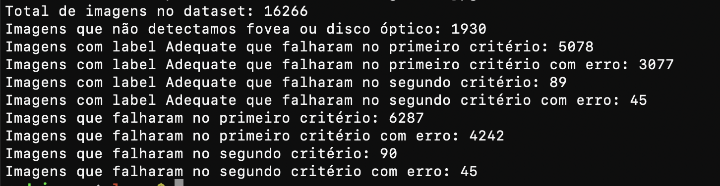
The image is in portuguese, but the main information follow:

• Out of the 16266 images on BRSet, we were not able to detect either fovea or optic disc for 1930 (due to limiting the confidence level to 0.5)
• 5078 images failed on the first criteria, i.e., the optic disc-nasal edge distance was smaller than one disc diameter.
• 89 images failed on the second criteria, i.e., the fovea-temporal edge distance was smaller than two disc diameters.

By taking a closer look at it, the results feel weird, how are there over 5000 images mislabeled? But from the manual testing we performed, our algorithm does not seem to be wrong, even though mistakes may happen, some detections may be inaccurate. On the other hand, most of the errors were made involving the optic disc, which is the eye structure we have a stronger model for detection, and our geometric algorithm has proven to work.

I took this results to my advisor, without having much confidence on how to use this on our paper, that’s when she came up with the idea of joining everything in a table and generating some better statistical analysis. After disagreeing with some of the columns she proposed, I came up with the final table:

image_id	quality_label	od_confidence	fovea_confidence	disc_diameter	od_center_x	od_center_y	fovea_center_x	fovea_center_y	nasal_distance	temporal_distance	od_fovea_angle
BRSet image ID	Inadequate, if fails on Image Field parameters, Adequate otherwise	Confidence of optic disc detection	Confidence of fovea detection	Optic disc bbox width	X Center coord for optic disc	Y Center coord for optic disc	X Center coord for fovea	X Center coord for fovea	Distance from OD to nasal edge	Distance from fovea to temporal edge	Rad angle between fovea and OD centers

We generated those data for all images on BRSet in which we were able to detect fovea or optic disc, and saved it to a .csv file. Now, we are using it to generate histograms and analyze the results obtained, with a full distribution for the dataset.

Data distribution analysis

Finally, we are able to generate some graphics and better visualize the results obtained. First of all, we plotted two histograms analyzing the distribution of the distances obtained, first between the optic disc and the nasal edge, second between the fovea and the temporal edge.

To better visualize, we have normalized the distances according to the disc diameter measure, so that we can explicitly see the image field criteria failing or going according to the data. Secondly, we have filtered the dataframe, using only images that had a higher confidence than 75% for fovea detection, and a higher confidence than 80% for optic disc detection. The histogram is also based on the density, and not absolute data.

The results follow:

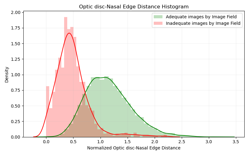Histogram evaluating the distance between OD and Nasal Edge

As we can see from this first graphic, most part of the inadequate images are actually on the correct region, with a distance between the optic disc and nasal edge below 1 disc diameter. A small portion of the data actually presents a value higher than 1, which we may assume that was considered inadequate by the other two criteria. However, a big part of adequate images actually do present that same distance below 1 disc diameter, suggesting that our first analysis was indeed correct, if the algorithm and methodology is working as expected, and the dataset does present a big number of wrongly attributed labels for Image Field criteria.

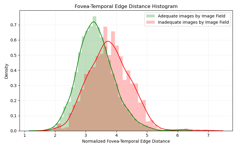Histogram evaluating the distance between Fovea and Temporal Edge

For this second plot, we do not have much to analyze. Most data are correctly labeled according to our methodology, and even though some mistakes are clearly happening, we are not taking it into consideration. Inadequates image must be labeled that way for failing in another Image Field criteria.

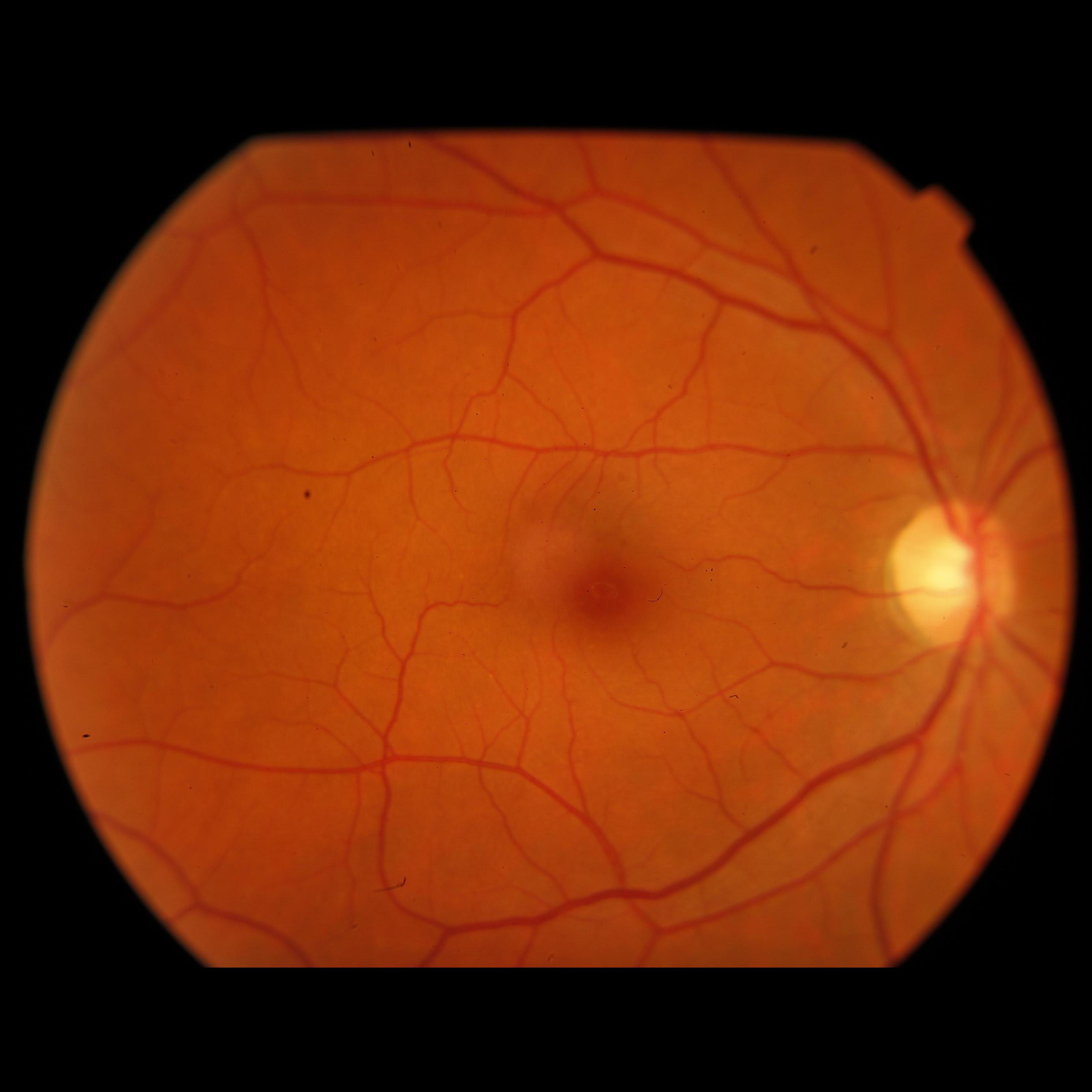
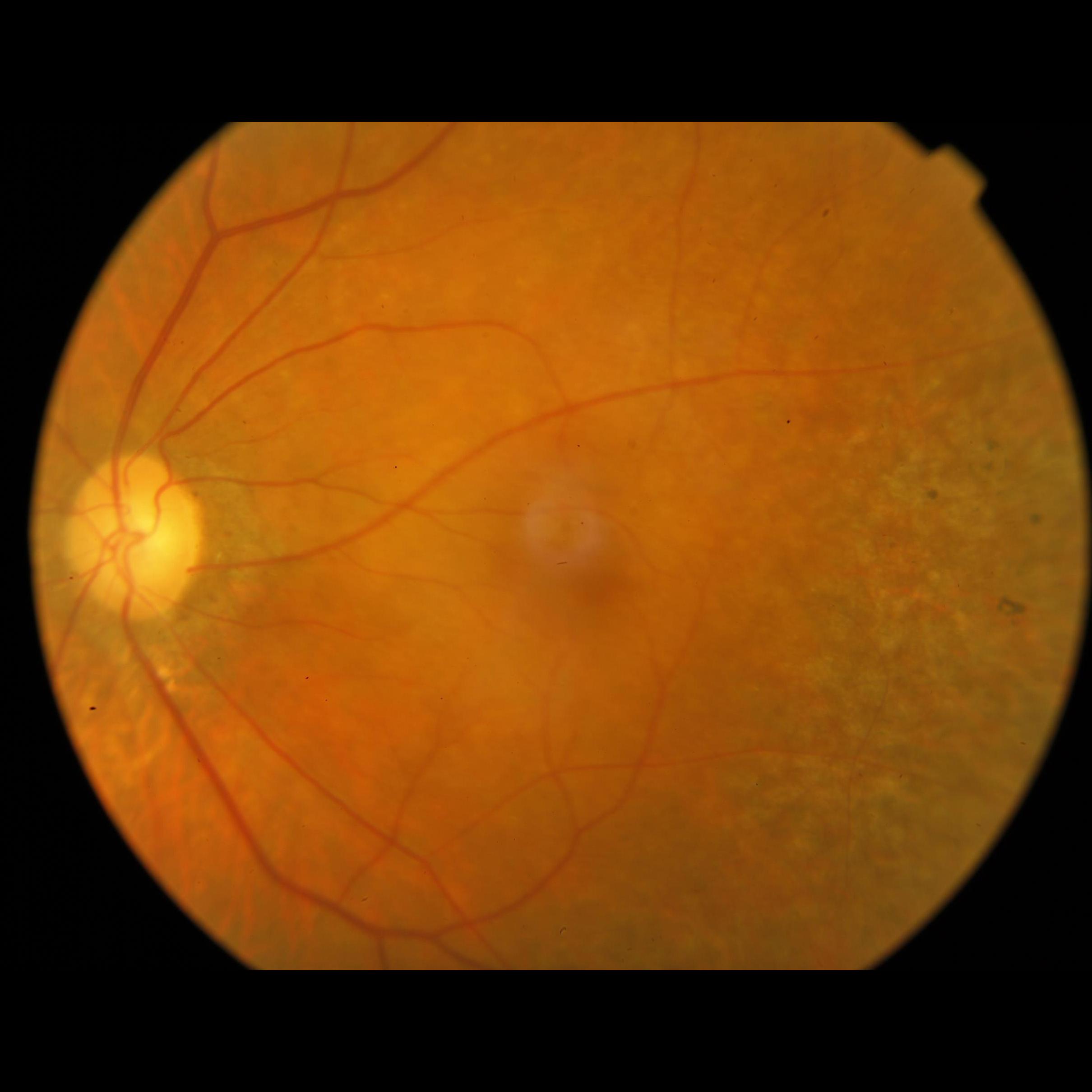
We have also analyzed how the images compare one to another, depending if its adequate or inadequate for Image Field, when both images have problems being closer to the nasal edge than 1DD. But as it turns out, both images look pretty much the same, having clearly an issue with this distance, and both should be considered inadequate. Below, you can see two images, the first one labeled adequate, and the second one labeled inadequate, both considering only Image Field definition.

Next Steps

For now, we have only analyzed those two histograms, but the data distribution is already super strong and well defined, and clearly points to where we thought it would: the dataset is mislabeled, according to its definitions. As for the next steps, I will send the results obtained here to my advisor and check if there are other analysis we should run, and also check if I should re-run the same analysis, but considering not counting images that are inadequate from another criteria (such as illumination, focus and artifacts), which are, for now, counted as “Adequate”, since it does not present Image Field problems.

We have also started writing a research paper for SIBGRAPI, as I mentioned before, and the paper due date was continued for July 31rd, so we will be spending the next few days writting it down.

• Understanding and studying the problem
• Choosing dataset
  • Preprocessing data
• Define training baseline
• Applying YOLO to detect Optic Disc (OD)
  • Obtaining the disc diameter (DD)
  • Obtaining distance from the OD to the Nasal Edge
• Detect Macular Center
  • Obtaining the distance from the Macular Center to the Temporal Edge
• Run statistical analysis on BRSet annotations
• Paper submission for SIBGRAPI
• Assessing visibility for the inferior and superior arcades

This post is used as a research checkpoint for the image quality assessment research on retinal fundus images, supervised by professor Nina S. T. Hirata, from the Institute of Mathematics and Statistics at the University of São Paulo (IME USP). The project is supported by USP/MCTI/Softex/Motorola.