[IQA #2] Detecting optic disc on retinal images with YOLO

In this post, we will be exploring how to apply YOLO using the Ultralytics Library, in order to detect the optic disc on retinal images, using the dataset that was built on the last post.

Defining training baseline

For all training, we have used Adam as an optimizer and trained for 40 epochs. We chose two different baselines, in order to evaluate the model performance in two scenarios, on precision, recall, mAP50 and mAP50-95, the standard Ultralytics metrics.

All models were trained on the same machine, using a NVIDIA RTX A5000 GPU, with 24GiB memory.

Baseline 1

In this baseline context, we have just divided our dataset normally, as if we were training a classifier. About 70% of the data were used for training, 15% for testing and 15% for validation, and shuffled the data using seed=42. With that, we got 443 images for validation and 445 images for testing.

Baseline 2

Since the BRSet dataset, our main dataset to evaluate, has no bounding boxes annotations, we wanted to see how the model would perform with data that it has never seen nor are simmilar to the ones we are feeding it during training. With that in mind, we have separated the Messidor dataset, that has 460 images, from the other datasets we are using, and defined that as our test set. The rest of the data were separated on 80% of the images for training and 20% for validation, using the same seed as before.

Results

We have trained the model for both scenarios described above, using the same configuration. With that, we were able to achieve nice results, that are shown on the tables below.

• Table 1: Results on baseline1

Metric	Test Result	Validation Result
Precision	0.987	0.975
Recall	0.995	0.993
Mean Average Precision mAP50	0.989	0.991
Mean Average Precision mAP50-95	0.877	0.887

• Table 2: Results on baseline2

Metric	Test Result	Validation Result
Precision	0.993	0.976
Recall	0.993	0.992
Mean Average Precision mAP50	0.989	0.989
Mean Average Precision mAP50-95	0.879	0.879

For what we are able to observe with the results obtained, the model seems to be performing just fine in order to detect the optic disc. Not only that, but the curves obtained from the Ultralytics run seem to be really good.

It is also important to observe the images and check if the results also match what we were expecting, and see if this model is actually useful. Since we do not aim to flood this post with images, specially with graphics, you can see the validation predictions for both baselines, respectively, in some examples as follow:

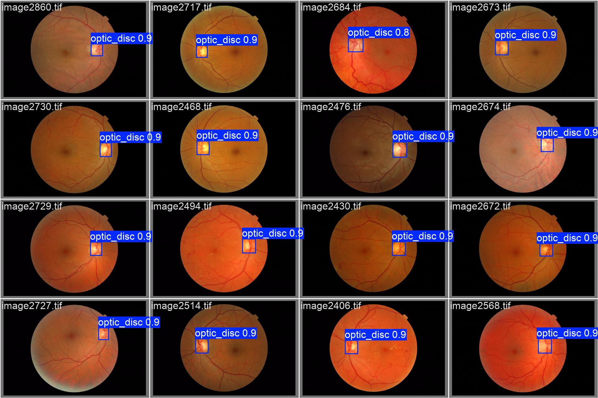
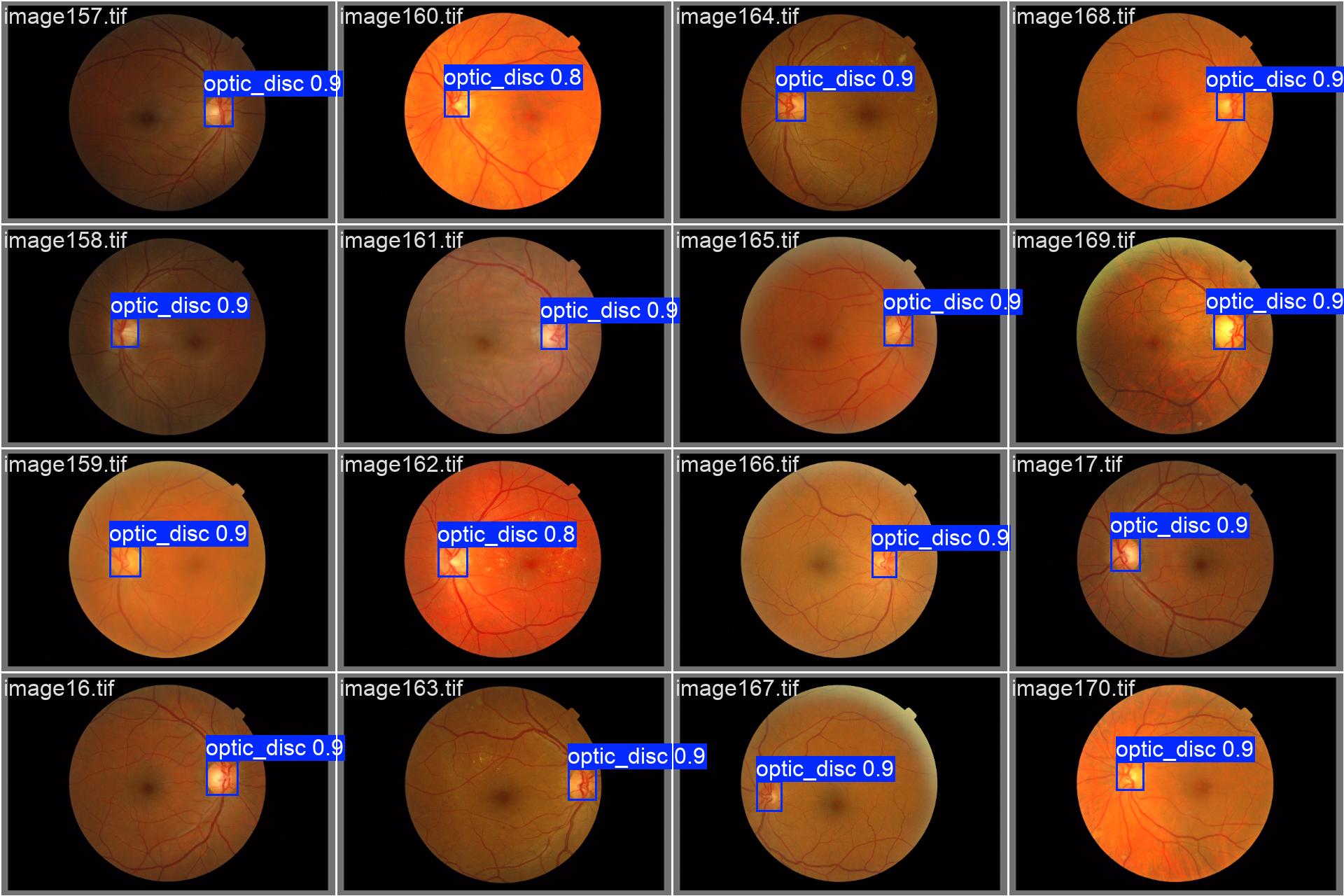
From what we are able to observe, the model seems to be performing great, and should be enough for our optic disc detection task.

Applying the model to obtain useful information

We have defined the following function, in order to run the model, trained with Ultralytics, on a given image:

def getCoordinates(imagePath, model):
    _, fileName = os.path.split(imagePath)
    imageName, _ = os.path.split(fileName)

    destPath = './src/data/images'

    model.predict(imagePath, save_txt=True, project=destPath, name=imageName)

    results = model(imagePath)
    results[0].save(filename=os.path.join(destPath, fileName), labels=True, line_width=2)

    return results

With that, we are able to obtain some important features from the model trained, on the results object returned. Suppose that our model actually works perfectly fine, our work now is, as explained on the first IQA post, obtain the disc diameter (DD), represented by the horizontal optic disc diameter, and check the distance from the optic disc to the nasal edge.

When looking at a retinal image, in most of the images, and the ones we are actually interested, the optic disc is located at the right or left side of the image, not centered. With that in mind, the retinal nasal edge is the retinal edge closer to the optic disc, i.e., if the optic disc is at the right side of the retinal image, then the right corner of the retinal is the nasal edge, and simmilarly to the left side.

Using results to solve the first metric

Knowing that, we are now able to detect the optic disc using our model and get its center coordinates. If the x coordinate obtained is bigger than the center of the image, we know that the optic disc is located on the right side, otherwise, it is located on the left side. This algorithm probably will be improved, knowing that, on some images, the retinal area is not fully centered. The DD is actually easily obtained from the results object, since it also returns the bounding box width. Not only that, we can also obtain the height of the center of the optic disc, also using the results object.

Now that we know which side is the nasal edge and we know the DD value, we can leave from the nasal corner of the optic disc (by using x = x_center + (width/2), if nasal edge is on the right side, x = x_center - (width/2) otherwise) and walk towards the nasal edge, by increasing or decreasing x. Note that, when doing that, we are assuming that the y coordinate from the center of the optic disc is located at the center of the retina, and getting a small error should be fine.

In order to detect when we have reached the nasal edge, we binarize the image, using a threshold value of 10, getting a image composed only by the retina (as white) and the background (as black). When we reach black on the binarized image, we got to the nasal edge. We could assure that the nasal edge occurs in the most extreme white point on the nasal side, but that would require detecting the edge itself or using a O(NxM) algorithm to explore the whole image matrix, which is not worth.

Next Steps

From what we have seen on the last topic, the optic disc detection may still face some issues, that will further be analyzed and reviewed, in order to see if it is necessary to refactor the code in any parts. But, for now, the results seem to be working as expected, and were approved by my advisor.

• Understanding and studying the problem
• Choosing dataset
  • Preprocessing data
• Define training baseline
• Applying YOLO to detect Optic Disc (OD)
  • Obtaining the disc diameter (DD)
  • Obtaining distance from the OD to the Nasal Edge
• Detect Macular Center
  • Obtaining the distance from the Macular Center to the Temporal Edge
• Assessing visibility for the inferior and superior arcades

This post is used as a research checkpoint for the image quality assessment research on retinal fundus images, supervised by professor Nina S. T. Hirata, from the Institute of Mathematics and Statistics at the University of São Paulo (IME USP). The project is supported by USP/MCTI/Softex/Motorola.